As the name suggest, this is an essential pipeline in data science workflow that involves exploration and understanding of data in order to determine the value of the attached variable, how they interlink and correlate with each other. In order to attain flexibility and rapid exploration process, I would share my workflow which involves a mixture of both R and Python programming language. To become a good data scientist, it is essential to get very comfortable with any of these 2 languages mostly Python as it is the most used in job practices and has a huge community of developers. I would suggest you expose yourself to be able to use both languages. A good knowledge of their syntax would give a major headway to work efficiently as a data scientist and a machine learning practitioner.
The goal of EDA is to help us understand our datasets better, in order to achieve this, the following base features must be handled:
- Names and number of variables observed
- Level of data missingness
- Presence of outliers
- Variable types and class
- Determine predictor variables and outcomes
- Split variables into continuous/categorical classes
For this first part of EDA series, the first line of action for a data scientist after data collection or before data wrangling, predictive analytics or machine learning, focus on data visualisation for EDA which is a very powerful tool often neglected considering the ease it brings to understanding data. The second part of this series would be using distribution, probability and some statistical test package to explore our data better. To achieve our goal today we would be using R-Studio and the following packages: Mice for missing data exploration and imputation; Reticulate for using both R and python objects in the same environment; on the python library side, we would be using Pandas for dataframe manipulation and analysis; then Seaborn and Matplotlib for visualisation.
Using the heart disease dataset captured on a Cleveland hospital database available on Kaggle. Note, this datasets have been deidentified and cannot be traced back to patients in any form for privacy and confidentiality purposes.
We import our dataset into R using read.csv and ensure a copy is available for python as an object.
getwd()## [1] "/Users/lade/Documents/Tosin_R_root"head(hrt)## age sex cp trestbps chol fbs restecg thalach exang oldpeak slope ca thal
## 1 63 1 3 145 233 1 0 150 0 2.3 0 0 1
## 2 37 1 2 130 250 0 1 187 0 3.5 0 0 2
## 3 41 0 1 130 204 0 0 172 0 1.4 2 0 2
## 4 56 1 1 120 236 0 1 178 0 0.8 2 0 2
## 5 57 0 0 120 354 0 1 163 1 0.6 2 0 2
## 6 57 1 0 140 192 0 1 148 0 0.4 1 0 1
## target
## 1 1
## 2 1
## 3 1
## 4 1
## 5 1
## 6 1r.hrt.dtypes## age int32
## sex int32
## cp int32
## trestbps int32
## chol int32
## fbs int32
## restecg int32
## thalach int32
## exang int32
## oldpeak float64
## slope int32
## ca int32
## thal int32
## target int32
## dtype: objectr.hrt.shape## (303, 14)Read your data guidelines or labeled notes thoroughly to understand what your data is trying to achieve and methods through which they were captured in order determine data completeness or missingness. Using R mice package we can check and visualise our data missingness as seen below. Check data summary using R object. R is know to produce more useful diagnostic outputs than python.
str(hrt)## 'data.frame': 303 obs. of 14 variables:
## $ age : int 63 37 41 56 57 57 56 44 52 57 ...
## $ sex : int 1 1 0 1 0 1 0 1 1 1 ...
## $ cp : int 3 2 1 1 0 0 1 1 2 2 ...
## $ trestbps: int 145 130 130 120 120 140 140 120 172 150 ...
## $ chol : int 233 250 204 236 354 192 294 263 199 168 ...
## $ fbs : int 1 0 0 0 0 0 0 0 1 0 ...
## $ restecg : int 0 1 0 1 1 1 0 1 1 1 ...
## $ thalach : int 150 187 172 178 163 148 153 173 162 174 ...
## $ exang : int 0 0 0 0 1 0 0 0 0 0 ...
## $ oldpeak : num 2.3 3.5 1.4 0.8 0.6 0.4 1.3 0 0.5 1.6 ...
## $ slope : int 0 0 2 2 2 1 1 2 2 2 ...
## $ ca : int 0 0 0 0 0 0 0 0 0 0 ...
## $ thal : int 1 2 2 2 2 1 2 3 3 2 ...
## $ target : int 1 1 1 1 1 1 1 1 1 1 ...source_python(file="EDA_cat.py")
print_categories(hrt)summary(hrt)## age sex cp trestbps
## Min. :29.00 Min. :0.0000 Min. :0.000 Min. : 94.0
## 1st Qu.:47.50 1st Qu.:0.0000 1st Qu.:0.000 1st Qu.:120.0
## Median :55.00 Median :1.0000 Median :1.000 Median :130.0
## Mean :54.37 Mean :0.6832 Mean :0.967 Mean :131.6
## 3rd Qu.:61.00 3rd Qu.:1.0000 3rd Qu.:2.000 3rd Qu.:140.0
## Max. :77.00 Max. :1.0000 Max. :3.000 Max. :200.0
## chol fbs restecg thalach
## Min. :126.0 Min. :0.0000 Min. :0.0000 Min. : 71.0
## 1st Qu.:211.0 1st Qu.:0.0000 1st Qu.:0.0000 1st Qu.:133.5
## Median :240.0 Median :0.0000 Median :1.0000 Median :153.0
## Mean :246.3 Mean :0.1485 Mean :0.5281 Mean :149.6
## 3rd Qu.:274.5 3rd Qu.:0.0000 3rd Qu.:1.0000 3rd Qu.:166.0
## Max. :564.0 Max. :1.0000 Max. :2.0000 Max. :202.0
## exang oldpeak slope ca
## Min. :0.0000 Min. :0.00 Min. :0.000 Min. :0.0000
## 1st Qu.:0.0000 1st Qu.:0.00 1st Qu.:1.000 1st Qu.:0.0000
## Median :0.0000 Median :0.80 Median :1.000 Median :0.0000
## Mean :0.3267 Mean :1.04 Mean :1.399 Mean :0.7294
## 3rd Qu.:1.0000 3rd Qu.:1.60 3rd Qu.:2.000 3rd Qu.:1.0000
## Max. :1.0000 Max. :6.20 Max. :2.000 Max. :4.0000
## thal target
## Min. :0.000 Min. :0.0000
## 1st Qu.:2.000 1st Qu.:0.0000
## Median :2.000 Median :1.0000
## Mean :2.314 Mean :0.5446
## 3rd Qu.:3.000 3rd Qu.:1.0000
## Max. :3.000 Max. :1.0000Using R’s DataExplorer package, find the attached report on our dataset that gives a rapid overview of the current state of our data. This can be very useful for a fast workflow
DataExplorer::create_report(hrt)table(is.na.data.frame(hrt))##
## FALSE
## 4242md.pattern(hrt)## /\ /\
## { `---' }
## { O O }
## ==> V <== No need for mice. This data set is completely observed.
## \ \|/ /
## `-----'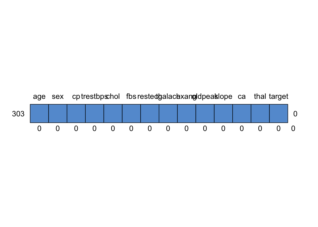
##     age sex cp trestbps chol fbs restecg thalach exang oldpeak slope ca
## 303   1   1  1        1    1   1       1       1     1       1     1  1
##       0   0  0        0    0   0       0       0     0       0     0  0
##     thal target
## 303    1      1 0
##        0      0 0
v2 <- vis_miss(hrt)
v3 <- gg_miss_var(hrt)
plot_grid(v2, v3, labels = "AUTO")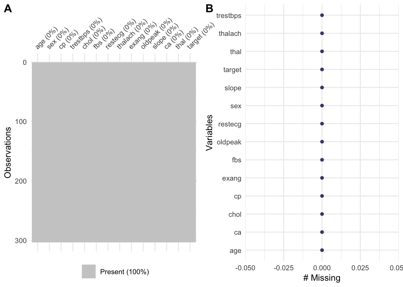
As seen above our dataset has no missing values
sns.distplot(r.hrt['chol'])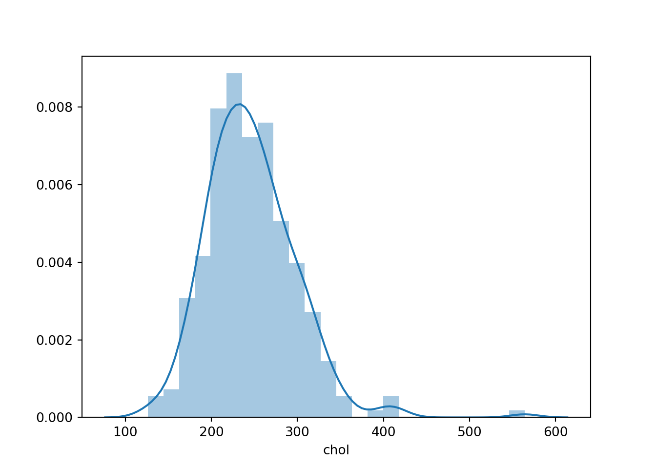
The above plot simply tells us that cholesterol measure is at its highest observation between 200 and 300
colnames(hrt)## [1] "age" "sex" "cp" "trestbps" "chol" "fbs"
## [7] "restecg" "thalach" "exang" "oldpeak" "slope" "ca"
## [13] "thal" "target"sns.jointplot(x='age',y='chol',data=r.hrt, kind='reg')## <seaborn.axisgrid.JointGrid object at 0x129132450>plt.show()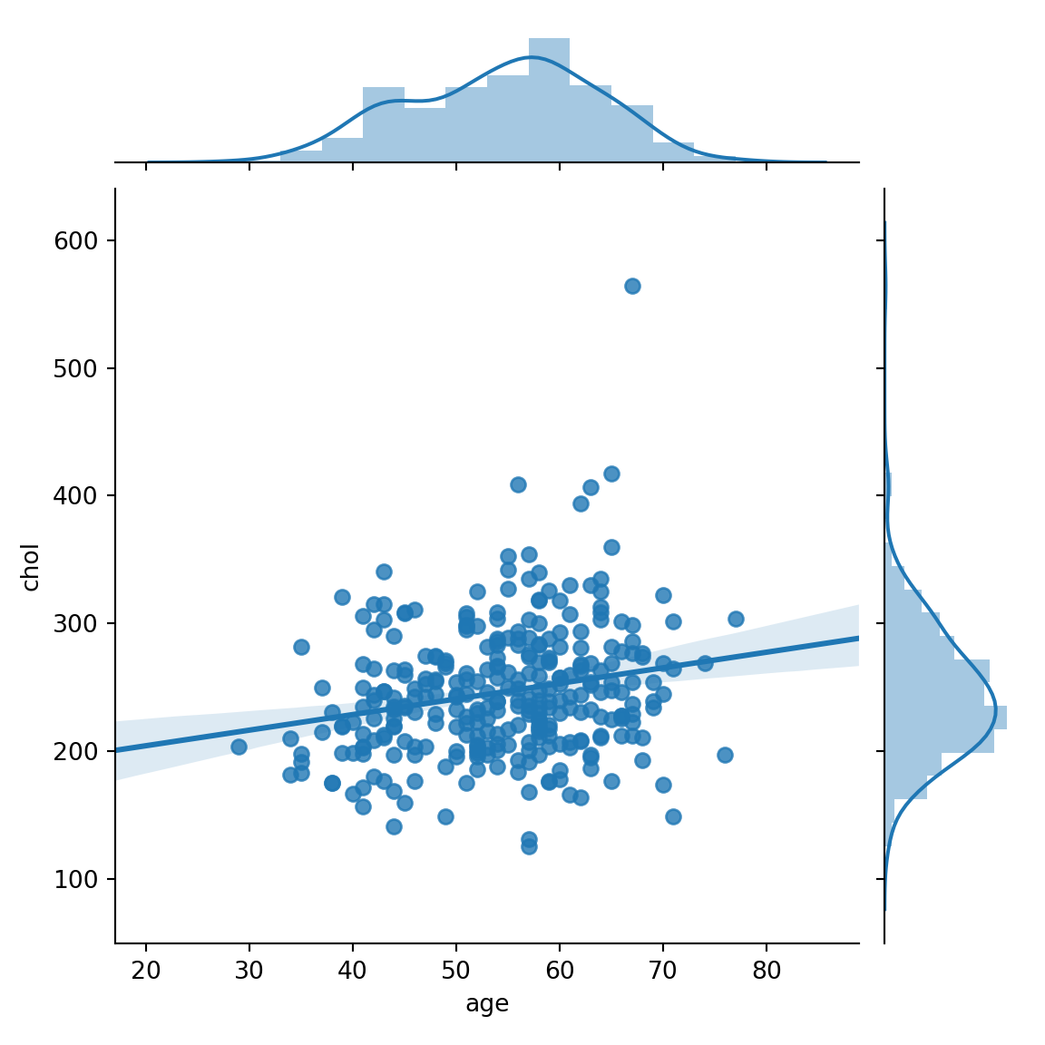
The distribution plot above allows us to compare the population age against cholesterol which is observed more in the older population than in the younger population.There is also a visible correlation as the fitted lm indicates that we can have a continuous prediction of possible outcome.
sns.jointplot(x='age',y='chol',data=r.hrt, kind='kde')## <seaborn.axisgrid.JointGrid object at 0x12f9704d0>plt.show()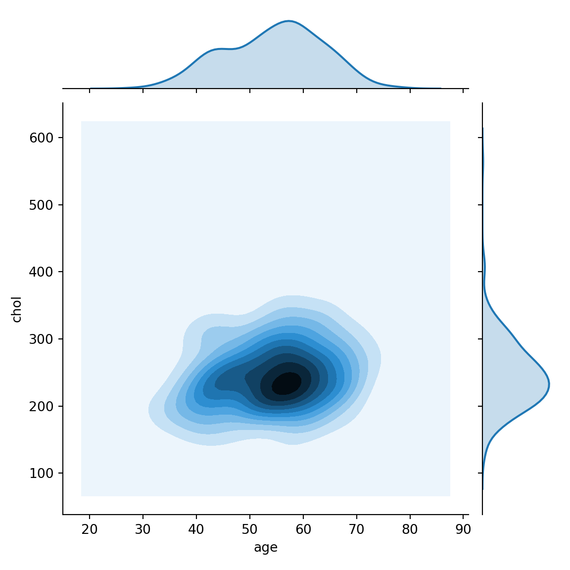
Compared to the previous jointplot, the above plot simply confirms the ideology of cholesterol concentration been higher in the older population than in the younger population.
sns.pairplot(r.hrt)## <seaborn.axisgrid.PairGrid object at 0x12f79eed0>plt.show()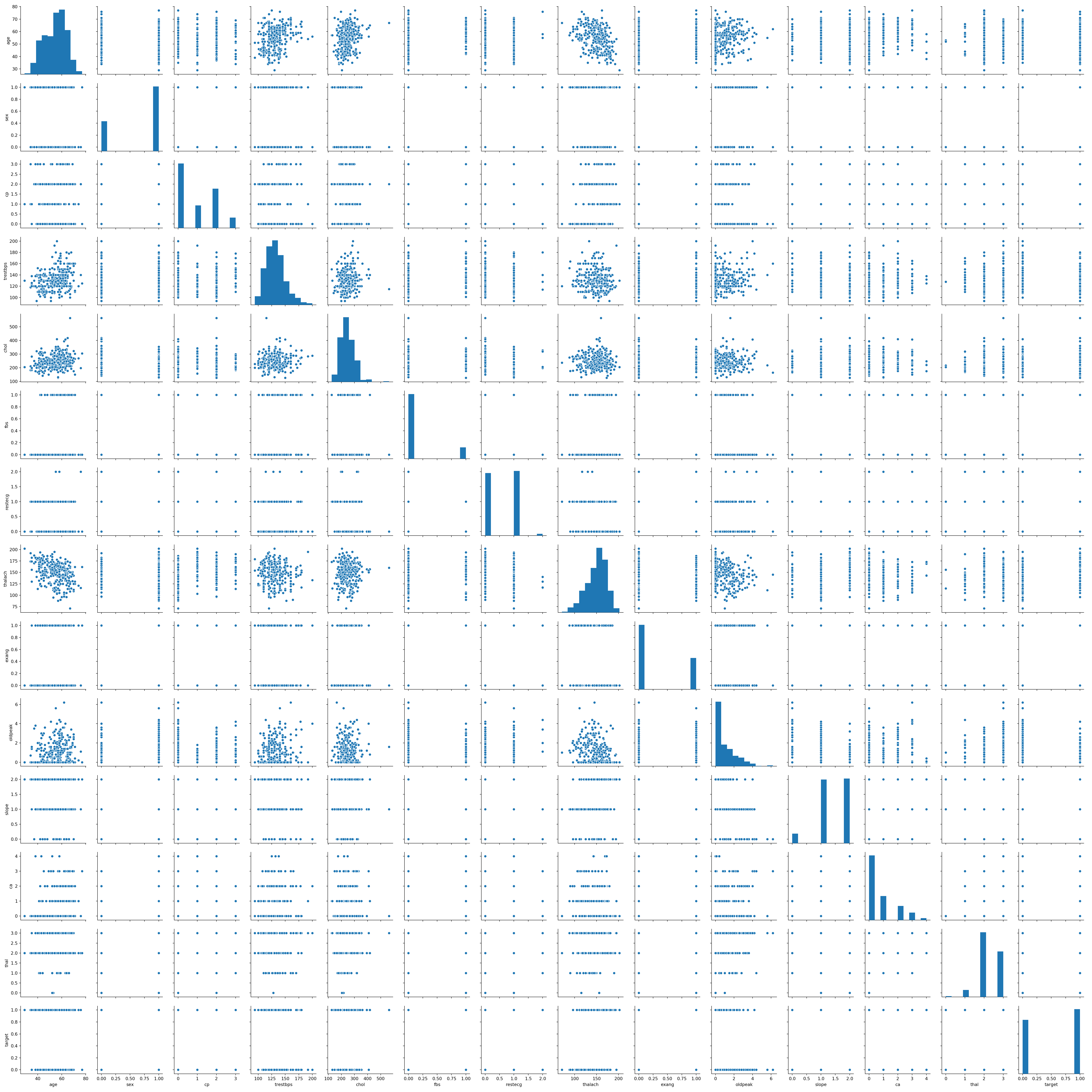
This is the fastest way to see through a dataset and explore the correlations between variables as well as visualising datatypes (categorical or continuous) and visualising their distributions. It is best to use a pairplot of the dataset as a whole in order to have a complete view.
sns.violinplot(x="sex", y="target", data=r.hrt, palette="rainbow")
plt.show()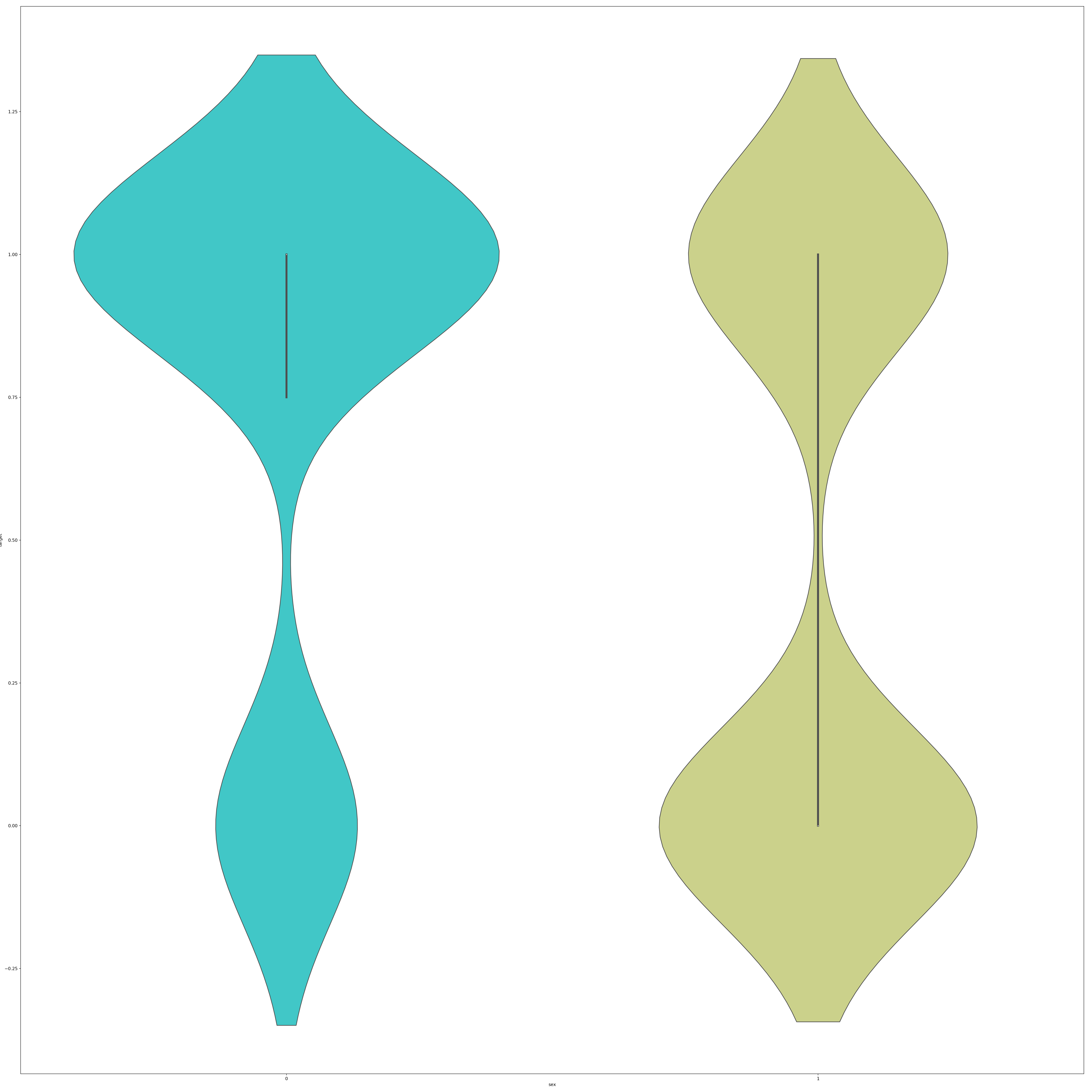
This final plot is known as a violin plot which shows that the captured data has the female population exhibiting the target outcome more than the male population. That is, the female population would have a higher tendency of been affected with a heart disease but not statistically confirmed or proven.